At first glance, JPEG (lossy) compression for images and mixing in audio engineering don't seem to have much in common. JPEG throws away data to shrink file sizes, an equalizer (EQ) reshapes sound to make a track hit harder. Under the hood, both operate on the same underlying concept of frequencies and I've combined both ideas in my Image EQ.
Recommended Pre-reading: https://weitz.de/dct/
JPEG transforms image pixel data into spatial frequency components, then gets rid of the information a viewer won't miss. An audio EQ transforms sound into frequency components, then lets you boost or cut them with faders. It's very similar math, but different goals in each of their applications.
I first ran into signal processing in the frequency domain back in 2021, doing a class project on the Discrete Sine Transform (DST) and image compression. We built MATLAB code that converted images to frequency space, zeroed out the high-frequency data (high frequencies that humans can't interpret), and dropped the file size while keeping the image recognizable. Just like how musically bass tones are low frequencies, and treble sounds have high frequencies, different "frequency bands" that make up an image encode different information. Low frequencies are where big spatial information is encoded, and high frequencies encode fine detail like texture. Data at certain high frequencies is imperceptible to the human eye. That's just a rough approximation though, I can't fully characterize the way the different frequencies change an image so I encourage you to play around with the Image equalizer on your own to get an intuition.
JPEG is an image format that can compress photos into smaller sizes. It does this using a close relative of the DST, the Discrete Cosine transform (DCT). The same core idea - decompose an image into basis patterns encoding different frequencies but with different handling of boundaries that makes it better suited for typical image data. Dr. Edmund Weitz has created one of the best explainers of the DCT that I've encountered, I highly recommend checking it out. You'll see how a small set of (linearly independent) basis signals combine to reconstruct any image, and why we can throw away certain information while keeping the core information in an image.
As I played around with music production I was learning about how to EQ and mix vocals. Just as an off thought one day I wondered, what would an EQ for an image look like? Instead of a single operation to discard frequencies for compression, what if you could grab the "bass" and "treble" of an image and drag them around with faders on a mixing board?
The DCT and JPEG Compression
Read through the DCT Explainer for a much better picture (or check out this video by computerphile) but in short, the Discrete Cosine Transform converts spatial information into frequency information. This transform is reversible, meaning that if we have the frequency information we can perfectly reconstruct the original pixels.
The 8×8 grid approach that JPEG uses breaks an image into 8×8 pixel blocks, then decomposes each block into a linear combination of these 64 basis functions:
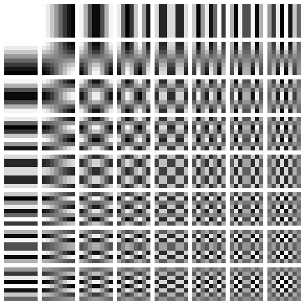
The top left tile is a solid color: this is the DC component (no fluctuations, just a flat value). It's mapped to a coefficient representing the average brightness. As you move one tile to the right or one tile down, you can see a fluctuation, from bright to dark across the span of the tile. Moving further right, or further down, this brightness oscillation becomes faster (and thus oscillates more within the span of the tile). The rows and columns preserve a similar relation to each other: one tile over or one tile down has a higher horizontal/vertical frequency than the preceding tile.
Any 8x8 block of pixels can be represented as a weighted sum of these 64 patterns (where the weights are the DCT coefficients). This works because the patterns are orthogonal: each captures something independent from the other patterns. These 64 blocks of 8x8 pixels can be combined to form ANY 8x8 block of pixels, but you can't create one of these basis blocks from any combination of any of the other basis blocks. Think of it like having 3 linearly independent vectors in a 3D vector space, you can combine and scale the three vectors (\(\hat{x}\), \(\hat{y}\), \(\hat{z}\)) in any way to create any other vector in that space (e.g. \(\langle 4, 7, 3\rangle = 4 \hat{x} + 7\hat{y} + 3\hat{z}\)), but you can't recreate a basis vector simply from the other basis vectors. No matter how you scale or combine the x- and y-direction basis vectors, you'll never get them to point in the z-direction.
The lossy compression of JPEG exploits a key principle of our visual perception. The low frequency bands of an image in the DCT transformed space contains broad shapes, lighting, large-scale gradients. Most of the energy of an image clusters in the low-frequency coefficients towards the top-left corner. The high frequency data on the right and bottom of the transformed image contains things like noise, sensor grain, and other rapid and sharp transitions. These are artifacts that don't contribute much to our visual understanding of the image, so we can get rid of them. JPEG operates in 8x8 pixel blocks: repeat this for every block in the image, apply some entropy encoding (to pack the remaining data even more efficiently), and you've got a JPEG.
EQing (Equalizing) Audio
The best explanation of EQ I've encountered, by far, is this video by Posy on YouTube. Conceptually: sound is made up of pressure waves travelling in a medium, and audio signals encode this pressure wave information into a changing voltage signal (changing amplitude over time). This changing voltage signal can also be decomposed into the frequency domain (e.g. via the FFT), and in this frequency space we can play around with the signal to shape it to our desires. We can apply gains here, to the "coefficients" of the frequency decomposition: boost the bass frequencies, cut some of the mid-range, cut some of the treble. Once we've operated on this signal in the frequency domain, we convert it back to the time domain and have our adjusted signal.
When working with audio, a unit you'll encounter is the decibel:
\[\text{dB} = 20 \log_{10}(\text{gain multiplier})\]
A gain of 1× is 0 dB (no change). Gain of 2× is about +6 dB. Gain of 0.5× is about -6 dB. Another influence from human perception, we hear (and see) ratios, not absolute differences. This is logarithmic perception and it's a hell of a Wikipedia rabbit hole to go down and I highly recommend digging into the Weber-Fechner law.
Compression ≠ EQ
Just like in music production, compression and EQ aren't the same thing. (Different meaning here, audio compression reduces dynamic range, while image compression reduces file size, but the conceptual separation still holds). If JPEG is the image equivalent of a compressor (loosely), I wanted to play with the equivalent of an EQ.
This meant applying the DCT to the entire image all at once. JPEG uses an 8x8 transform: an 8x8 transform can recreate any 8x8 grid of pixels using 8×8=64 basis functions. For computational speed and simplicity, the image EQ automatically compresses to 128×128, which still results in a whopping 16,384 basis patterns.
Compression is a whole fun rabbit hole of itself to dig into, but here it's simply handled by the browser's canvas API.
ctx.drawImage(img, 0, 0, 128, 128);Even with this though, just going from 128×128 to 256×256 doubles N, meaning 8x the computation. This is why JPEG doesn't DCT the whole image but rather goes in 8x8 blocks, operating in the 64 basis functions of the 8x8 space.
For the 128×128 case (or the 256×256 case) the resulting spectrum is conceptually the same: for each of the (R)ed, (G)reen, and (B)lue channels in the original image, DC (the average brightness) lives in the top left, and high frequency in the bottom right.
For the EQ, once the compressed (resized) image is transformed to the frequency domain, we can apply the gains to the different spatial frequency bands based on the faders, and then transform back to the spatial domain.
The DCT image shows you the value of coefficients at different "frequencies", with a further radial distance from the top left DC corner representing a higher frequency. Mathematically:
\[f = \frac{\sqrt{k_x^2+k_y^2}}{\sqrt{2}N}\]
where \(f\) represents the "frequency" at a position \((k_x, k_y)\). For simplicity, I divvied this radial distance up into four bands: 0-15% for the low band, 15-40% is mid-low, 40-80% is mid-high, and 80-100% is "high". It wouldn't be realistic to have a fader for every one of the 16,384 basis patterns, this keeps it manageable and interpretable.
Computationally Expensive
It's still a hell of a computation though. A naive 2D DCT is O(N⁴): if you have an N×N pixel image, you have N² output coefficients, and need to sum over N² input pixels. At 256×256, that's over 4 billion operations per color channel.
This is where the DCT's separability lends a hand, you can decompose a 2D grid of basis patterns into a product of a horizontal 1D cosine and a vertical 1D cosine. That means we can compute the 2D transform as two passes of 1D transforms: first the rows, then the columns.
A single 1D DCT on N points requires O(N²) operations (N outputs, each summing N inputs). For an N×N image with N rows, the row pass is applied N times, N × O(N²) = O(N³). The column is another pass at O(N³), leaving the order of magnitude still at O(N³), still better than the O(N⁴) naive approach.
Visualizing the Image's Transform
Raw DCT coefficients have huge dynamic range: the DC component could be 50,000 while high frequency components are at 0.91. If the coefficients are mapped linearly to brightness all we'd see in the transform was a single bright pixel in the corner surrounded by black.
Thus, the brightness displayed is logarithmically scaled:
const displayValue = Math.log(1 + Math.abs(coefficient) / maxCoefficient * 255) * 30;Same as audio perception, log-scaling is how we reveal structure in our perception (the 30 at the end is a scaling constant for the visualization).
Try it out!
Go to ashish.is/developing/doodles/image-eq, you can use a standard test image by clicking DEMO (props to man.bmp), or upload your own, compress it, and see the transform in the R, G, and B channels. Look at the different patterns that emerge boosting the highs vs the lows, and the emergent visuals when you zero out other bands.